Image geometry and interpolation

Image interpolation techniques are used to enlarge or shrink images. They include nearest neighbor, linear, cubic, and bicubic. These techniques produce progressively better quality results as we go from the nearest neighbor to bicubic. However, they also place increasingly more computational demands as we go from the nearest neighbor to bicubic. Before we discuss these techniques, we will discuss a computationally simple but an ineffective approach to image interpolation.

Reducing the image size by row and column removal

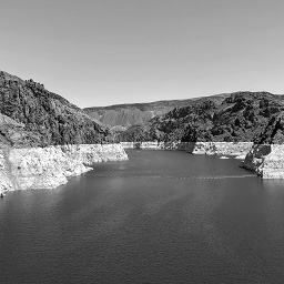
Consider an $n \times n$ image and we would like to shrink this image to half its original size. In other words, the shrunk image would be $n/2 \times n/2$. A computationally simple but crude approach is to simply drop the odd numbered rows and odd numbered columns from the original image. The process of producing a lower spatial resolution image from a higher spatial resolution image is called down-sampling. Shown below is a grayscale image of Hoover dam, which is a $404 \times 303$ image.

A grayscale image of the Hoover dam. The image size is 404 rows and 303 columns.

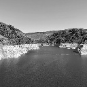
A down-sampled image of size $256 \times 256$ from the original $404 \times 303$ image is shown below.

A down-sampled image of the Hoover dam from the original image. The down-sampled image size is 256 rows and 256 columns.

Next, we generate the following down-sampled images from the $256 \times 256$ down-sampled image:

128 $\times$ 128
64 $\times$ 64
32 $\times$ 32
16 $\times$ 16
8 $\times$ 8
4 $\times$ 4

Shown below are $128 \times 128$ and $64 \times 64$ down-sampled images. We do not show the other versions due to their smaller sizes.

A down-sampled image of the Hoover dam. The image size is 128 rows and 128 columns.

A down-sampled image of the Hoover dam. The image size is 64 rows and 64 columns.

Increasing the image size by row and column replication

We consider the problem of image enlargement or magnification. The process of producing a higher spatial resolution image from a lower spatial resolution image is called up-sampling. Nearest neighbor, linear, cubic, and bicubic interpolation techniques produce better quality images. But first we will demonstrate up-sampling using a computationally simple but crude approach. This involves simply replicating the rows and columns of the original image. For example, producing a $4 \times 4$ image from a $4 \times 4$ image requires replicating each row and each column. More specifically, we make a copy of the first row and place it right below the first row. We repeat the same process for the remaining rows. We use this image for the following process. We make a copy of the first column and place it immediately to its right. This process is repeated for the remaining columns.

Shown below are six images which are up-sampled from the following down-sampled images:

4 $\times$ 4
8 $\times$ 8
16 $\times$ 16
32 $\times$ 32
64 $\times$ 64
128 $\times$ 128

⊕ $An up-sampled image of the Hoover dam. The image is up-sampled to 256 $$\times$$ 256 from a 4 $$\times$$ 4 image.$
An up-sampled image of the Hoover dam. The image is up-sampled to 256 $\times$ 256 from a 4 $\times$ 4 image.

⊕ $An up-sampled image of the Hoover dam. The image is up-sampled to 256 $$\times$$ 256 from a 8 $$\times$$ 8 image.$
An up-sampled image of the Hoover dam. The image is up-sampled to 256 $\times$ 256 from a 8 $\times$ 8 image.

⊕ $An up-sampled image of the Hoover dam. The image is up-sampled to 256 $$\times$$ 256 from a 16 $$\times$$ 16 image.$
An up-sampled image of the Hoover dam. The image is up-sampled to 256 $\times$ 256 from a 16 $\times$ 16 image.

⊕ $An up-sampled image of the Hoover dam. The image is up-sampled to 256 $$\times$$ 256 from a 32 $$\times$$ 32 image.$
An up-sampled image of the Hoover dam. The image is up-sampled to 256 $\times$ 256 from a 32 $\times$ 32 image.

⊕ $An up-sampled image of the Hoover dam. The image is up-sampled to 256 $$\times$$ 256 from a 64 $$\times$$ 64 image.$
An up-sampled image of the Hoover dam. The image is up-sampled to 256 $\times$ 256 from a 64 $\times$ 64 image.

⊕ $An up-sampled image of the Hoover dam. The image is up-sampled to 256 $$\times$$ 256 from a 128 $$\times$$ 128 image.$
An up-sampled image of the Hoover dam. The image is up-sampled to 256 $\times$ 256 from a 128 $\times$ 128 image.

All image interpolation techniques will provide better results than the ones shown above.

Back to course home