Histogram equalization
Histogram equalization is a pixel intensity transformation technique. Each pixel in the original image is mapped to another value, including no change in the pixel value. This mapping is provided by the histogram equalization transformation function, which is computed using the cumulative distribution function (CDF) for the continuous case and probability mass function (PMF) for the discrete case.
Histogram equalization essentially transforms the pixel values of the source image such that the histogram of the resulting image has a uniform distribution. In other words, the histogram equalization stretches the intensity values so that the image is represented by all the intensity values. As an example, for an 8-bit image, the full range of intensity values is \([0..255]\). However, the pixel values in an image may encompass only a subrange of \([0..255]\).
For digital images, the histogram distribution after equalization is only approximately uniform given that we approximate integration with summation (i.e., substitute PMF for CDF) and round-off in the computations required as pixel values are integers. In the following, we illustrate the histogram equalization process using a synthetic image.
Consider the following synthetic 5-bit, \(16 \times 16\) image.
| 10 | 12 | 9 | 6 | 7 | 4 | 0 | 2 | 9 | 8 | 11 | 5 | 12 | 9 | 13 | 5 |
| 14 | 7 | 13 | 0 | 15 | 14 | 15 | 5 | 7 | 8 | 8 | 10 | 4 | 13 | 14 | 2 |
| 5 | 14 | 10 | 3 | 2 | 6 | 3 | 14 | 8 | 9 | 1 | 4 | 0 | 14 | 9 | 3 |
| 12 | 5 | 10 | 6 | 7 | 12 | 7 | 1 | 7 | 11 | 2 | 8 | 4 | 13 | 2 | 5 |
| 12 | 13 | 5 | 1 | 5 | 15 | 4 | 4 | 5 | 7 | 6 | 4 | 5 | 14 | 6 | 1 |
| 2 | 15 | 13 | 0 | 2 | 5 | 11 | 6 | 0 | 5 | 11 | 14 | 7 | 14 | 2 | 1 |
| 12 | 8 | 10 | 3 | 1 | 5 | 13 | 0 | 9 | 4 | 7 | 14 | 5 | 5 | 11 | 8 |
| 1 | 5 | 15 | 6 | 14 | 3 | 6 | 3 | 6 | 10 | 6 | 10 | 3 | 0 | 13 | 5 |
| 13 | 1 | 8 | 14 | 14 | 3 | 6 | 13 | 1 | 9 | 10 | 11 | 5 | 12 | 2 | 9 |
| 8 | 10 | 0 | 0 | 5 | 5 | 13 | 10 | 3 | 13 | 7 | 13 | 10 | 13 | 1 | 15 |
| 5 | 6 | 7 | 10 | 6 | 14 | 11 | 6 | 2 | 13 | 6 | 12 | 12 | 15 | 1 | 0 |
| 6 | 11 | 13 | 10 | 3 | 10 | 6 | 13 | 11 | 5 | 5 | 7 | 2 | 9 | 7 | 8 |
| 14 | 0 | 13 | 11 | 13 | 2 | 7 | 3 | 1 | 11 | 9 | 10 | 4 | 5 | 8 | 6 |
| 9 | 0 | 11 | 11 | 15 | 12 | 12 | 15 | 6 | 8 | 5 | 11 | 5 | 10 | 11 | 0 |
| 14 | 10 | 15 | 2 | 1 | 14 | 9 | 9 | 5 | 13 | 3 | 13 | 8 | 5 | 9 | 0 |
| 0 | 14 | 8 | 3 | 15 | 10 | 2 | 2 | 8 | 14 | 13 | 11 | 8 | 12 | 8 | 14 |
Since this is a 5-bit grayscale image, the range of intensity values is [0,31]. However, the intensity values are confined to the narrow range [0,15] by design. See the image histogram below.
![Histogram of a 5-bit synthetic image before histogram equalization. The pixel values are in the range [0,15]](/csci4150/course-content/spatial-domain-processing/histogram-equalization/graphics/histogram-before-equalization.png)
| Original pixel value \((r)\) | Frequency \((f_r)\) | Relative frequency \((\frac{f_r}{MN})\) | Cumulative frequency (CDF) | Pixel value after histogram equalization | Rounded pixel value after histogram equalization |
|---|---|---|---|---|---|
| 0 | 15 | 0.0586 | 0.0586 | 1.8164 | 2 |
| 1 | 13 | 0.0508 | 0.1094 | 3.3906 | 3 |
| 2 | 15 | 0.0586 | 0.1680 | 5.2070 | 5 |
| 3 | 13 | 0.0508 | 0.2188 | 6.7812 | 7 |
| 4 | 9 | 0.0352 | 0.2539 | 7.8711 | 8 |
| 5 | 28 | 0.1094 | 0.3633 | 11.2617 | 11 |
| 6 | 19 | 0.0742 | 0.4375 | 13.5625 | 14 |
| 7 | 14 | 0.0547 | 0.4922 | 15.2578 | 15 |
| 8 | 17 | 0.0664 | 0.5586 | 17.3164 | 17 |
| 9 | 14 | 0.0547 | 0.6133 | 19.0117 | 19 |
| 10 | 18 | 0.0703 | 0.6836 | 21.1914 | 21 |
| 11 | 16 | 0.0625 | 0.7461 | 23.1289 | 23 |
| 12 | 12 | 0.0469 | 0.7930 | 24.5820 | 25 |
| 13 | 22 | 0.0859 | 0.8789 | 27.2461 | 27 |
| 14 | 20 | 0.0781 | 0.9570 | 29.6680 | 30 |
| 15 | 11 | 0.0430 | 1.0000 | 31.0000 | 31 |
Shown in the first column are the distinct intensity values in the image that we desire to histogram equalized. Frequency of occurrence of pixel intensities are shown in the second column. The third column is the relative frequency, which is obtained by dividing the relative frequency by the number of pixels in the image. For the \(16 \times 16\) image, \(M=16, N=16\).
![Histogram of a 5-bit synthetic image after histogram equalization. The pixel values are stretched to the full range [0,31]](/csci4150/course-content/spatial-domain-processing/histogram-equalization/graphics/histogram-after-equalization.png)
Histogram equalization can be efficiently implemented using the lookup table:
| Original pixel value | Pixel value after histogram equalization |
|---|---|
| 0 | 2 |
| 1 | 3 |
| 2 | 5 |
| 3 | 7 |
| 4 | 8 |
| 5 | 11 |
| 6 | 14 |
| 7 | 15 |
| 8 | 17 |
| 9 | 19 |
| 10 | 21 |
| 11 | 23 |
| 12 | 25 |
| 13 | 27 |
| 14 | 30 |
| 15 | 31 |
The first column shows the distinct pixel values in the original image. The corresponding values in the right column are the pixel intensities after the histogram equalization. For example, the pixel value 5 in the original image is transformed to 10 in the histogram equalized image. Though not shown in the above table, in general, the histogram equalization transformation function may map multiple pixel values in the original image to the same pixel value in the histogram equalized image.
Next, we use the histogram equalization transformation function represented by the two-column table above to equalize the histogram of the original image. The image pixel values in the histogram equalized image are:
| 21 | 25 | 19 | 14 | 15 | 8 | 2 | 5 | 19 | 17 | 23 | 11 | 25 | 19 | 27 | 11 |
| 30 | 15 | 27 | 2 | 31 | 30 | 31 | 11 | 15 | 17 | 17 | 21 | 8 | 27 | 30 | 5 |
| 11 | 30 | 21 | 7 | 5 | 14 | 7 | 30 | 17 | 19 | 3 | 8 | 2 | 30 | 19 | 7 |
| 25 | 11 | 21 | 14 | 15 | 25 | 15 | 3 | 15 | 23 | 5 | 17 | 8 | 27 | 5 | 11 |
| 25 | 27 | 11 | 3 | 11 | 31 | 8 | 8 | 11 | 15 | 14 | 8 | 11 | 30 | 14 | 3 |
| 5 | 31 | 27 | 2 | 5 | 11 | 23 | 14 | 2 | 11 | 23 | 30 | 15 | 30 | 5 | 3 |
| 25 | 17 | 21 | 7 | 3 | 11 | 27 | 2 | 19 | 8 | 15 | 30 | 11 | 11 | 23 | 17 |
| 3 | 11 | 31 | 14 | 30 | 7 | 14 | 7 | 14 | 21 | 14 | 21 | 7 | 2 | 27 | 11 |
| 27 | 3 | 17 | 30 | 30 | 7 | 14 | 27 | 3 | 19 | 21 | 23 | 11 | 25 | 5 | 19 |
| 17 | 21 | 2 | 2 | 11 | 11 | 27 | 21 | 7 | 27 | 15 | 27 | 21 | 27 | 3 | 31 |
| 11 | 14 | 15 | 21 | 14 | 30 | 23 | 14 | 5 | 27 | 14 | 25 | 25 | 31 | 3 | 2 |
| 14 | 23 | 27 | 21 | 7 | 21 | 14 | 27 | 23 | 11 | 11 | 15 | 5 | 19 | 15 | 17 |
| 30 | 2 | 27 | 23 | 27 | 5 | 15 | 7 | 3 | 23 | 19 | 21 | 8 | 11 | 17 | 14 |
| 19 | 2 | 23 | 23 | 31 | 25 | 25 | 31 | 14 | 17 | 11 | 23 | 11 | 21 | 23 | 2 |
| 30 | 21 | 31 | 5 | 3 | 30 | 19 | 19 | 11 | 27 | 7 | 27 | 17 | 11 | 19 | 2 |
| 2 | 30 | 17 | 7 | 31 | 21 | 5 | 5 | 17 | 30 | 27 | 23 | 17 | 25 | 17 | 30 |
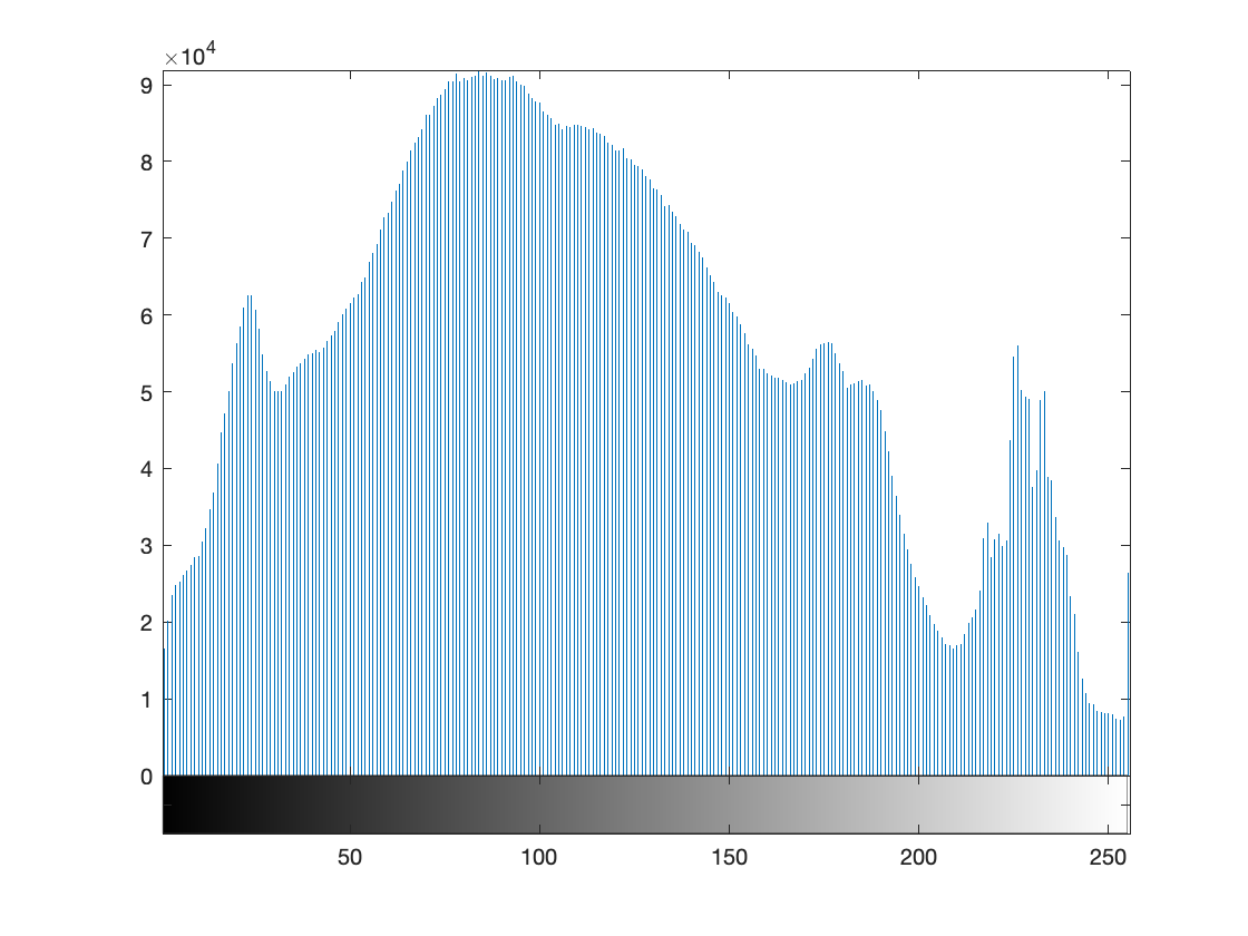
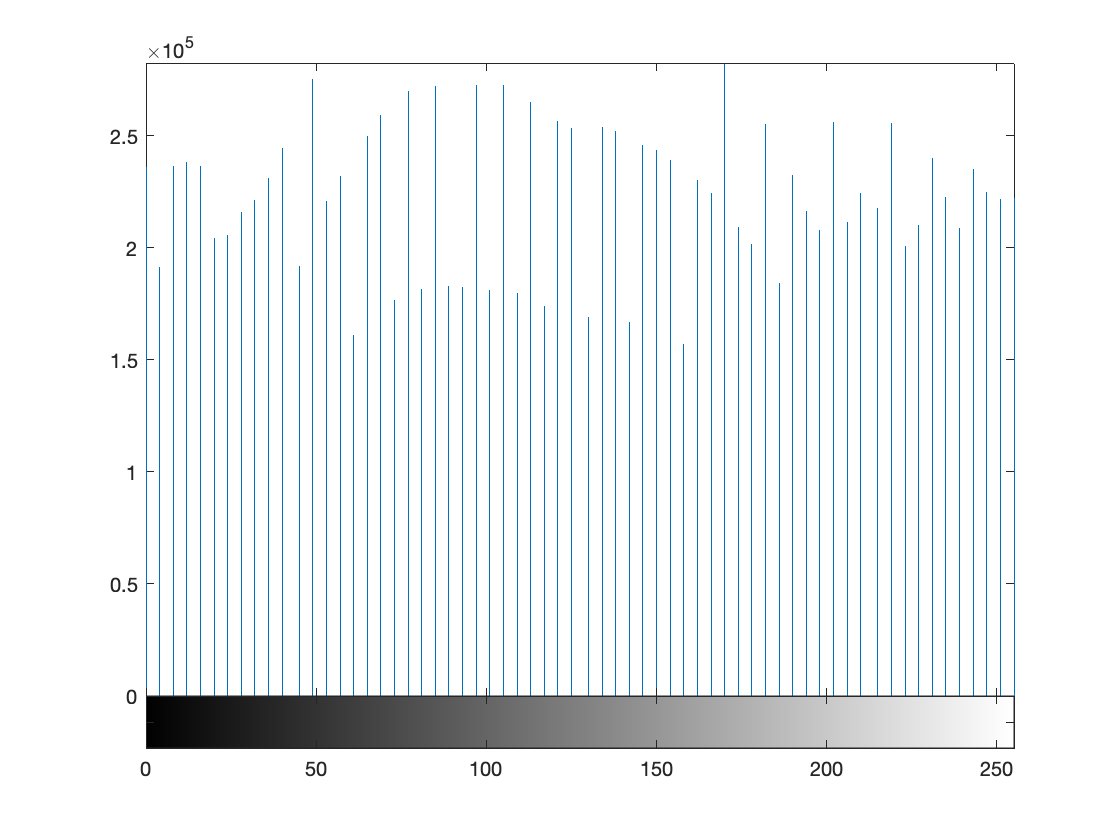
Shown below are two histograms of a real image. The first one is the histogram before equalization and the second is the histogram after equalization. You can clearly the see effect of histogram equalization on the shape of the histogram.
| Histogram before equalization of a real image of size \(2120 \times 2252\) | Histogram of the image after equalization |
|---|---|
 |
 |